Projects

Oxygen -18

xingu river

Sediment Budget Analysis

sediment sources

mud mounds

Tectonic Deformation

Stream Channel Responses
Fall 2019
Mentor: Dr. Julie Bryce
Applications of δ18-O to Mid-Latitude Alpine Glaciers for Paleoclimatic Research: Examples from the Wind River Range, WY
Introduction
Stable isotopes in water are affected by meteorological regimes and atmospheric conditions that can provide a unique identifier of their origin. Analyzing the composition, concentration, and stratigraphic distribution of δ18O in ice cores is an effective method for paleoclimate reconstructions that has been demonstrated in numerous sites, most famously in the ice sheets of Antarctica and Greenland, but in small alpine glaciers as well (e.g., the high Andes). δ18O in well-preserved ice can be used as a proxy for temperature, and with ancillary geochemical data for piecing together a record of hydroclimate change. Prior to the research that was conducted in the Wind River Range (WY), mid-latitude glaciers were thought to have minimal potential to reveal reliable information on paleoclimate. The uncertainties are generally attributed to meltwater percolation effects and the broad range of oxygen isotope abundances as a response to higher seasonal variability in these regions. In this paper, I discuss: (a) the basic processes and controls of oxygen isotope speciation, (b) paleoclimate applications of δ18O to polar ice sheets, (c) the motivation behind applying δ18O geochemistry to ice cores from the Wind River Range, (d) the calibration and geochronology methods specifically used in these mid-latitude glaciers, and (e) key evidence of the Little Ice Age from Wind River ice cores, including a the development of a refined age-model created from δ18O and electrical conductivity measurements, and a transfer-function used to establish mean annual temperature changes using δ18O.
Fractionation & Oxygen Isotopes
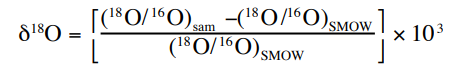
Figure 1: Equation for delta18-O. (Clark & Fritz, 1997)
To investigate the application and use of δ18O glacial ice, we must first understand the basic process that allows different isotopes of oxygen to occur from fractionation and how these isotopes are measured. The species of oxygen isotopes is a function of temperature and is strongly influenced by certain meteorological and hydrological processes.
Isotopic Fractionation
Isotopes of the same element have different masses, resulting from a difference in the number of neutrons, which helps to account for varied reaction rates that can facilitate fractionation or partitioning of a certain species in a reservoir. Physiochemical fractionation is characterized by faster reaction rates in lighter nuclei than heavier isotopes due to their smaller bond strength. Heavier isotopic species are more commonly partitioned into a more condensed phase, such as the solid phase in mineral-solution reactions or the aqueous phase in vapor-liquid interactions (Clark & Fritz, 1997).
Oxygen Isotopes
Stable isotopes are measured as ratio of the two most abundant isotopes for a given element. Measured ratios are compared to a reference standard to produce a difference expressed as parts per thousand (per mil, ‰). For oxygen isotopes, 18O has a terrestrial abundance of 0.204% and 16O has a terrestrial abundance of 99.796%. Thus, the ratio is about 0.00204. Ratios determined in a given sample are referenced to SMOW, the Standard Mean Ocean Water. Oxygen isotope fractionation is mass-dependent, which means that it is proportional to the mass gradient or difference. Lighter molecules have greater translational velocities, which allow them to emerge from a liquid surface more easily and evaporate more readily than the heavier molecules. Hydrogen fractionations are related to oxygen isotopes in precipitation, however hydrogen is greater because the mass difference is greater. Despite the fact that only 10% of evaporated moisture from the oceans reaches the continents, a variety of partitioning pathways can occur by process such as rainfall, re-evaporation, and snow and ice accumulation. Oxygen and hydrogen isotope behavior can usually be be very confidently predicted through the meteoric water line (MWL) (Clark & Fritz, 1997). The MWL describes the astonishing correlation of δ18O and δ2H in freshwater reservoirs on a global scale. For example, isotopically depleted waters are commonly found in high latitude cold regions while those that are enriched by evaporation are located in warmer regions in the tropics. Typical values of δ18O for Greenland fall in the range of -30 to -35‰, while ice in Antarctica can exhibit δ18O values as low as -50‰ (Clark & Fritz, 1997).
Meteorological Controls
Temperature regulated mechanisms have potentially large effects on the stable isotopic composition of precipitation. These mechanisms include the Latitudinal Effect, Continentality Effect, and Altitude Effect (Clark & Fritz, 1997).
Latitudinal Effect
In general, precipitation at higher latitudes produce more negative δ18O. δ18O Temperature gradients are -0.6‰ for δ18O per degree of latitude for North American continental stations (Clark & Fritz, 1997). Water can exist in several phases, including solid (ice), liquid (water), and gas (vapor), and temperature and pressure changes can alter the phases. Strong seasonal variability and the range of temperatures related to latitude (especially in places like North America) offer a significant control on the isotopic evolution of vapor and precipitation, and therefore broad differences in δ18O should be expected between areas like Florida versus New Hampshire .
Continental Effect
Isotopic composition of water vapor evolves as it moves from its ocean source inland. This is caused by topographic effects and temperature extremes that are common for continental interiors that aren’t moderated by marine influences (Clark & Fritz, 1997). As a result, continents can strong seasonal variations in temperature. This effect is described by continentality (k), where the average annual range in temperature is related to the latitudinal angle. This relationship is given by the equation: K = (1.7ΔT / sin(ϕ+10)) – 14 (Clark & Fritz, 1997).
Altitude Effect
Temperature and altitude are normally inversely related: as elevation increases, temperature declines, and this can be seen in the vegetation and snowlines on many mountains. Depletion of 18O varies between -0.15‰ and -0.5‰ per 100 m rise in altitude (Clark & Fritz, 1997). At high altitude, sublimation – the process by which snow is converted to vapor – and other modifying processes can also influence the δ18O (Naftz et al., 2002). The orographic precipitation influence on oxygen isotope fractionation is evident where mountains force air masses up to a cool altitude that can facilitate condensation and precipitation. Thus, precipitation on the leeward side of a topographic high point will be isotopically lighter than on the windward side.
Process Related Variability: Rain
The process of rain cloud formation and ultimate releasing of these condensed particles has a particular influence on the variability of oxygen isotopes.
Raleigh Distillation
Raleigh distillation is a process through which isotopically enriched rain is formed and falls as wet deposition from a diminishing vapor mass and this residual vapor (f) is progressively depleted as a result. R = R0 fα-1 (Clark & Fritz, 1997) This process leads to changes in the isotopic composition of rainfall across long distance storm tracks, in spite of a common starting point or moisture source.
Rain Formation
The isotopic evolution of precipitation during rainout is determined by temperature. Since rain is formed when a vapor mass is cooled adiabatically by rising to a region in the atmosphere with lower pressure, it eventually reaches a temperature at which there is 100% humidity (i.e., the dew point), allowing it to condense and fall as rain or snow (Clark & Fritz, 1997). Thus, the temperature within the cloud helps to determine what species of O is partitioned and condensed and not the surface or local temperature. However, given the difficulty in monitoring internal cloud temperatures, relationships of 18O variability are deduced using local mean temperature data.
Rainout
Research has shown that δ18O of ice may be controlled by δ18O of precipitation, which is dominated by moisture supply and storm trajectories. Rainout is involved in the process where a trajectory (wind patterns, weather systems, etc.) directs an air mass away from its evaporative source and over a continent to higher latitudes and potentially altitudes. The air mass experiences several episodes of cooling and loss of water vapor by precipitation along this path, successively distilling the heavy isotopes from the vapor and become progressively depleted in 18O and 2H (Clark & Fritz, 1997).
Significance
Analyzing the composition, concentration, and stratigraphic distribution of δ18O in ice cores is an effective method for paleoclimate reconstructions. Isotope studies made on ice cores are widely referenced in Quaternary studies, and similar to marine isotope records made from foraminifera, are considered to be important tracers of global environmental changes (Ruddiman, 2001). In a typical ice core, isotopically enriched summer layers alternate with more depleted winter horizons (Clark & Fritz, 1997). Using this relationship, δ18O in wellpreserved ice can be used as a proxy for temperature, which is one of the most important variables for understanding climate history, especially in the Quaternary. These δ18O are sometimes combined with other ice measurements that be used to learn about atmospheric composition, volcanic processes, and more.
Glacial Studies
The application of oxygen isotopes as a proxy for paleoclimate was led by the pioneering work of scientist Willi Dansgaard, one of the namesakes for Dansgaard-Oeschger cycles (Ruddiman, 2001). Following the release of several comprehensive publication on the subject of oxygen and hydrogen isotopes in ice starting in the 1950’s, a progressively improved understanding of these isotopes was bestowed upon the scientific community, which led to greater application and improved interpretations. The Greenland Ice-Core Project (GRIP) was established in the early 1990’s and since that time, foundational papers have been produced detailing the variability of δ18O in precipitation and ice records in response to local environmental conditions and global atmospheric interactions. Two of these early papers together have been cited more 3000 times (Grootes et al., 1993, Johnsen et al., 2001). One prominent discovery was rapid climatic changes in the Pleistocene, which are the abrupt changes in δ18O (several per mille each) and temperature (signifying a rapid warming and slower cooling) that make up the Dansgaard-Oeschger cycles. The cycles occurred approximately every 1500 years and their causes have been debated (Ruddiman, 2001). One possibility is ice sheet instability and breakup, while another revolves around changes in greenhouse gases in the atmosphere. Another key finding from Greenland was the occurrence of big changes in deglacial and Holocene climate, such as the Younger Dryas and the 8,200 year event. In particular, the Younger Dryas appears as a big and abrupt shift to lower δ18O in Greenland Ice (Grootes et al., 1993). This led scientists to conclude that cold periods could affect the earth even during a major phase of deglaciation. The relationship of oxygen isotope fractionation with respect to mean annual temperature has been recognized by correlations observed in Greenland ice cores over long time scales in the Pleistocene and has even been linked to specific snow storm events and their temperatures more recently. The Antarctic record in the southern hemisphere also has been explored for temperature data using δ18O, and these cores go back farther in time than the Greenland data. These distinct and relatively clear patterns in temperature and oxygen isotopes have only been observed in the polar regions; mid-latitude sites in the USA provide limited insights into these anomalous systems, which will be discussed more in relation to the Wind River Range (Naftz et al., 2002).
Despite the surge of oxygen isotope studies on the polar ice sheets, minimal efforts have been made to investigate the variability of δ18O in mid-latitude alpine glaciated regions. This is why I will discuss only a handful of papers pertaining to the Wind River Range that were published mostly in the late 1990’s.

Figure 2: EOS Article. Vol. 73, No. 3, January 21, 1992.
Applications in Mid-Latitude Glaciers in the Wind River Range
For sites in the mid-latitudes, δ18O of ice can be more difficult to interpret, and may be more closely associated with the average annual air temperature than precipitation delivered by storm paths (Naftz et al., 2002) since mid-latitudes have much higher seasonal temperature variability than polar regions. Prior to the research that was conducted in the Wind River Range, mid-latitude glaciated regions were considered to have minimal potential to reveal reliable information on paleoclimate. However, the data produced from USGS scientists in these inaugural studies document some similar patterns with respect to other ice cores obtained from higher latitudes and elsewhere.
January, 1992, a scientific newspaper (EOS) published a short column about a USGS drilling project team that had successfully collected a 160 m long ice core from Fremont Glacier in 1991. This drilling project had been active in climate research studies on temperate glaciers in the Wind River Range since 1988, mostly in an effort to determine the chemical quality of the atmospheric deposition as a consequence of upwind sources of pollution and particulates. The chemical composition of glacial ice can provide a useful record of constituents previously suspended in the atmosphere that are deposited in the wet (precipitation of rain and snow) and dry (dust particle fallout) forms. In the 1980’s, the national atmospheric deposition program (NADP) was established by the federal government to monitor wet deposition of atmospheric pollution. This record is relatively short and the what is found in downwind glacial ice can extend the record back in time beyond the time of the NADP database. The ice coring project was in partnership with several official organizations including the Shoshone and Arapaho Indian tribes, PICO, BLM, and the WY Water Development Commission to legitimize the importance of atmospheric non-point source pollution.
Wind River Geographic Setting
The Wind River Range is located in central Wyoming and is the highest and longest mountain system in the state, containing the highest peak (Gannett Peak at 13,804 ft) and extending 80 mi with an approximate N-S strike within the greater Rocky Mountains. The greatest concentration of glaciers for all of the Rockies, including 7 of the 10 largest glaciers in the contiguous USA, are found in the Wind Rivers. The location and geography of the Wind Rivers is important to Rockies hydrology. The continental divide spans the crest of the range and joins a third divide – the Green River headwaters - on the north end that creates a triple divide for the Columbia River watershed in the west, Missouri River in the east, and upstream Green River portion of the greater Colorado River basin. The glaciers studied in Wind Rivers include Knife Point, Gannett, and Upper Fremont Glacier. A study done in the nearby Absaroka Mountains investigated Galena Creek Glacier to compare to Upper Fremont. All four glaciers are situated on the eastern side of the Continental Divide.
Early Studies: Meltwater Percolation and Chronological Considerations
Meltwater production and percolation within ice bodies can create issues for paleoclimate studies in the mid-latitudes (Cecil et al., 1998). These effects may dampen seasonal δ18O signals and cause a shift to less negative δ18O values (Naftz et al., 1996). This issue was a big concern for the researchers trying to extract climate signals from the Upper Fremont Glacier ice core, even though care was taken to collect ice from the accumulation zone at high elevation, where meltwater should be minimized.

Figure 3: Concentrations of tritium in ice samples compared to depth from the Knife Point Glacier, representing the time between 1987-1980 and a 2.5m maximum depth. (Fig. 2, Naftz et al., 1991)
35-S and Tritium at Galena Creek Glacier
To distinguish between recent and older sections of ice and to test for meltwater contributions, an analysis of the abundance of 35S, a radioactive nuclide produced by cosmogenic rays, was used because of its very short halflife of 87 days (Cecil et al., 1998). Ice and meltwater represented in the core should have no 35S prior to 1940 and may contain very small amounts of 35S after 1980 (Cecil et al., 1998). 35S is quickly oxidized to form sulfate and it gets easily incorporated into glacial ice upon deposition. The meltwater composition of 35S in Galena Creek expressed a low value of about half of what would be observed in modern precipitation (5.4mBeq/L). Considering the short half-life, this suggested that recent melting had occurred from accumulation that was deposited within the last two years. In other words, the signal represents meltwater from recent precipitation, because there was no apparent contribution from older ice. This finding was important because it implied to the authors that Galena Creek glacier and Upper Fremont glacier were experiencing slow rates of ablation. Galena Creek ice was also analyzed for 3H, in order to distinguish between older and younger ice and to see if sources of meltwater percolate into and disrupts the ice stratigraphy. The values found in the Galena Creek Glacier were similar to modern precipitation, suggesting old meltwater contributions are insignificant in the ice record.
Atmospheric Deposition of Major Ions at Knife Point Glacier
To identify layers of ice that had not been contaminated by meltwater, the abundance of major ions left by atmospheric deposition was investigated in an ice core from Knife Point Glacier (Naftz et al., 1991). To minimize this risk of meltwater percolation interference, ice was again collected at elevations greater than 3500 m asl. The purpose of this study was to examine annual layer preservation, to see if Wind River glaciers could be accurately dated, and to determine if the chemical composition of the ice is related to wet deposition as opposed to atmospheric fallout (dust or dry deposition).
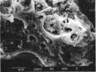
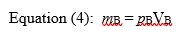
Figure 4: Photomicrograph of Mount St. Helen’s ash collected near Kellogg, Idaho on May 21, 1980 representing the vesicular structure of the ash grains. (Fig. 3, Naftz et al., 1991)
In order to use ice cores to reconstruct different aspects of climate or pollution history, a chronology of ice accumulation is necessary. However, several studies showed that the mid latitude glaciers did not preserve extensive laminations like those seen in high-latitude glaciers (Naftz et al., 1996). Knife Point contained a few prominent laminations, and this study focused on a short interval of time using a trench surface dug into the ice. Unlike some of the other Wind River glaciers, Knife Point showed annual layering marked by thin laminations of gray colored dust. A useful chronological marker was Mount St. Helens’ last eruption (1980), which dispersed copious volumes of ash into the atmosphere that is recognized in sediment or ice archives by ash with silica enrichment and the presence of vesicles. Geochemical analysis of these dust in Knife Point revealed a particular layer that was compositionally similar to the ash deposited by this Mount St. Helens eruption (Naftz et al., 1991). Another useful chronological marker was the appearance of trichlorofluoromethane (CCl3F). CCl3F is produced by industrial reactions and is not otherwise found in the naturally occurring environment. Beginning in 1931, humans began producing this compound. Where CCl3F concentrations were detectable in the ice, it indicated an age younger than 1931 (Naftz et al., 1991). The last time marker that was evaluated was tritium (3H). Nuclear weapons testing conducted in the 1950’s and 1960’s released large amounts of neutrons in the upper atmosphere that were subsequently bonded with other atmospheric isotopes and exposed to cosmogenic radiation via spallation to produce acute concentrations of unstable and radioactive isotopes, including 3H (as well as 36Cl). Following formation, these molecules then attached themselves to aerosols in the atmosphere resulting in ‘fallout’, or deposition as precipitation or dust, thus allowing the rapid elimination of these particles from the atmosphere. Geochemical records in ice cores document the distribution and abrupt reduction of radioactive nuclides in the atmosphere by deposition since nuclear weapons testing. The production and abrupt atmospheric concentrations of 3H and 36Cl can be used by as precise geochronometers since the concentrations on either side of the time of nuclear testing – pre and post 1950’s-1960’s – should be very low (Cecil et al., 1998). From the Knife Point glacier, the 3H record shows an increasing abundance with depth between known ages of 1980 to 1987 (Naftz et al., 1991).
From the major ion analysis, abundances of Ca, Mg, Na, Cl, and SO4 were measured and compared to wet deposition concentrations recorded by the NADP in Pinedale, WY. Of these elements, only Ca, Cl, and SO4 were positively correlated with NADP, although the sulfate correlation was still relatively poor. The authors argued that because the correlation exists, then meltwater must not be contaminating Knife Point glacier, and that long ice cores could provide a great deal of contaminant and climate history information.
Upper Fremont Glacier - Initial Chronology
Upper Fremont was most important for the USGS ice core studies, as it was the longest and oldest glacial record from the Wind Rivers. Several samples from the 160 m core were dated using radiocarbon. A majority of the dates produced from these samples yielded large uncertainties and were consequently discredited – except for one. A grasshopper leg found at 152 m was determined to be 1716-1820 AD (221 +/- 95 bp). This age, coupled with the knowledge of the exact species of the grasshopper, provided the ice core with at least one conclusive age to evaluate modern accumulation rates and climate history (Naftz et al., 1996). A number of other methods were used to build up the chronology of the Upper Fremont core. For example, the concentration of 36Cl was measured, which as discussed above, is related to nuclear weapons testing. The 36Cl peak was found at the 32 m depth (Cecil and Vogt, 1997). Using tritium, Cecil et al. found no evidence of meltwater contamination at depth in the Upper Fremont ice. 3H levels from the Upper Fremont glacier ice core displayed a marked peak at a depth of 29 m, exceeding 300TU. This boundary layer corresponds to when above ground nuclear weapons testing was most frequent in the early 1960’s (Naftz et al., 1996).
Evidence for the Little Ice Age Anomaly in δ18-O and nitrates

Figure 5: Relation of the d18O values with depth in the 160m Upper Fremont Glacier. Shaded section (100-150m depth) represents section of high-amplitude oscillations identified in the Upper Fremon Glacier ice-core record. (Fig. 5, Naftz et al., 1996)
δ18O measurements taken from the ice core extracted from Upper Fremont glacier revealed signatures consistent with the Little Ice Age (LIA) (Naftz et al., 1996). Within the Upper Fremont ice core, the average δ18O over the entire 160 m core was -18.9‰. Significant isotopic variations in the core are mostly in the lower part of the core, below 101.8 m depth, where the average δ18O value is -19.85‰. Overall, the core exhibits more negative δ18O and high amplitude oscillations of δ18O during the LIA, compared to as less variable δ18O after the LIA (Naftz et al., 1996). Radiocarbon dates from deep ice sections indicate that the more negative δ18O ice formed in the mid-1700’s to mid-1800’s. These ages correlate with temperature reconstructions done for Europe which correspond to the end of the LIA. Similar studies done on tree rings in the western US also confirm this was a cold period in North America (Naftz et al., 1996).
Greater δ18O variability shown in the deeper ice from the mid 1700-1800’s might represent conditions of either more summer precipitation (when δ18O are more positive) or more winter precipitation (when δ18O are more negative). Colder LIA summers could have also preserved the δ18O signal better by limiting seasonal melting (Naftz et al., 1996). The LIA and post-LIA oxygen isotope compositions in this core are further substantiated by comparing the δ18O composition to the famous Quelccaya ice core from the Peruvian Andes. Both cores exhibit more negative δ18O and high amplitude oscillations of δ18O during the LIA, as well as less variable compositions after the LIA (Naftz et al., 1996). Nitrate concentrations in the Upper Fremont Glacier were very low during the LIA, and low nitrate concentrations were observed in Greenland ice during glacial intervals. A possible explanation can be attributed to less nitrogen-fixing bacteria in the snow during these colder episodes. More positive δ18O and nitrate concentrations in the bottom 10 m of the core may be an effect of a basal meltwater layer and freezing/refreezing at the bedrock contact (Naftz et al., 1996).
Development of a Refined Age-Model using Electrical Conductivity

Figure 6: Nitrate concentration profile from UF core with depth (0-160m). (Fig. 3, Naftz et al., 1996)
Electrical conductivity (ECM), sulfate and chloride concentrations were measured for Upper Fremont ice core by Schuster et al. (2000), and the results were compared to chemical age dates and the 18O profile provided by the previous research to correlate acidic atmospheric fallout from volcanic events with core depth, in order to refine the chronological history of the Upper Fremont Glacier. ECM is a direct approach to measuring the acidity of ice. Particulate products of volcanic eruptions and anthropogenic industrial activities, such as sulfate and chloride, are acidic and get released into the atmosphere, eventually falling out by a wet or dry depositional process, accumulating in ice and increasing the electrical conductivity. Core samples from depths greater than 15m (below the firn layer, where ice was compact) consistently exhibited significant CL- and SO42- peaks where there is also a significantly high ECM signal. ECM can help detect events where evidence has been altered. For example, EDA and SEM measurements identified the Mount St. Helens ash layer in Knife Point glacier, about 4mi SE of Upper Fremont. This ash layer was not visible in the Upper Fremont ice core, suggesting meltwater may have removed ash particulates from the surface, only leaving behind the residual acidity that was detected by ECM. Schuster et al. (2000) outlined the elution sequence of major chemical components removed through meltwater percolation effects in glaciers (SO42- > NO3-, NH4+, K+, Ca2+, Mg2+, H3O+, Na+, Cl-). This represents the order in which major ions are removed from ice by meltwater during warm summer months, a process that mid-latitude glaciers are especially vulnerable to and has been observed in Wind River glaciers (Naftz et al., 1993). Thus, any preserved chemical signal in the ice may reflect a diminished fraction of what was initially deposited. The lower 10 m of core reflects enhanced chemical variability, similar to those observed in the 18O. Between 150-155m depth, Cl- concentrations exceed the highest Cl- concentration recorded in the rest of the core by more than two times. Elevated Cl- and no considerable ECM signal at this basal depth suggests the Cl- more likely originates from chemical interactions at the ice-bedrock interface and not atmospheric origins.
Schuster et al. (2000) expressed dissatisfaction with the rudimentary age model provided in Naftz et al., even noting the grasshopper leg radiocarbon age was only moderately credible because of a 95 yr error bar and failing to consider post-depositional movement within the core. Schuster et al. (2000) suggested that the chemical dates determined from 3H, 36Cl, and radiocarbon outlined in Naftz et al. (1993) provide a “preliminary” age-depth profile. This initial model predicted that deposition for the layer at 88 m depth occurred in 1881. This depth is coincident with the highest ECM signal, representing one of the largest volcanic events in history from the eruption of Krakatau in Indonesia in 1883. Atmospheric dust from this event was observed in North America just a few months after the eruption. Thus, the layer at 88m depth in Upper Fremont was deposited in 1883, instead of 1881. The second largest ECM peak in the core occurs at 123 m. The initial age model proposes an 1805 AD time of deposition. Another massive volcanic eruption occurred in Indonesia at Tambora in 1815, releasing ash into the atmosphere that was observable in North American and England skies for nearly 6 months almost immediately after the eruption. Thus, the layer at 123m depth in Upper Fremont was deposited in 1815, instead of 1805. The refined agemodel is based on these two prominent dates and ECM signals correlating to the 27 most recent and significant volcanic (Figure 8, Figure 9). This refined profile is in good agreement with radiocarbon age of the grasshopper, yielding 1736 A.D. deposition at 152m depth.

Figure 7: Profile of a 999-point running average of ECM data with depth (0-160m) from the UF glacier showing a decrease in variance at 108m. (Fig. 4, Schuster et al., 2000)
δ18O variance increases abruptly in the lower half of the Upper Fremont ice core beyond 108m depth, previously determined to be a response to LIA climate. However, due to the coarse (20 cm) sampling resolution for δ18O, the end of the LIA was indeterminate. Comparing ECM and 18O profiles, ECM values show a coincident abrupt shift to decreased variance at this boundary. The refined age model yields an age of 1845 A.D. at this depth, representing the LIA termination and abrupt shift to warmer temperatures. Confidence and prediction limits suggest the time taken to complete the LIA climatic shift to present-day climate was about 10 years – meaning LIA termination in mid-latitude alpine regions of North America happened over a relatively short time-scale.

Figure 8: Plot of reported volcanic events and isotopic age dates used to generate a polynomial fit for an age-depth profile of the UF ice core. (Fig. 6, Schuster et al., 2000)
Using δ18-O to Reconstruct Temperature Changes with Transfer Functions (Naftz et al., 2002)
There have been a few studies that attempt to extract additional information from the Upper Fremont δ18O record, in spite of its shortcomings. In this study of Naftz et al. (2002), a transfer function, a statistical relationship relating temperature of snow storms to the δ18O in the deposited snow/ice, was developed and ultimately applied to Upper Fremont using the revised Schuster et al. (2000) age model. Transfer functions are unforgiving and must be developed for a specific site. This study was done by setting up a weather station with accurate sensors that recorded hourly weather metrics over several years, including temperature and snow accumulation depth for every storm. Transfer functions were made for four time intervals, each spanning a year. In the years where temperature and δ18O are related, the slope of the linear relationship changes. These slope changes may be explained by convective cloud droplets and reevaporation during late spring or summer snow events. Redeposition of snow and removal of snow by wind can influence the snow depth measurements and isotopic composition at the surface of the glacier. Wind sensors on the glacier indicate dense early season snows are less susceptible to removal by wind, while colder temperatures after October generate less dense snow that can be transported by wind more easily. All of these processes are relevant for making the transfer functions effective as describing temperature changes in the distant past.
Two ice cores from two different sites on the Upper Fremont glacier collected in 1991 and 1998 both show a significant isotopic enrichment of δ18O in the upper 40m, indicative of a warming trend in annual temperatures from the early 1950’s to early 1990’s (Figure 10). To reconstruct the annual temperature from ice core data collected at UFG in 1998, a transfer function from site-specific air temperature and δ18O values in snow deposited on the UFG was applied. The plot of these annual temperature changes with respect to δ18O values from the 1998 core suggests 3.5°C of warming from the mid-1960’s to early 1990’s (Figure 11). The same transfer function was applied to depths of 102150m in the 1991 core and yielded a positive 5°C change in temperature between the end of the LIA (mid1800’s) to early 1900’s. These reconstructions are substantially higher than the global average of 1°C of warming for the 20th century. However, similar changes in mean annual temperature over this time period has been calculated from select high-altitude, high-latitude polar regions, suggesting the mid-latitude alpine glaciers are extremely vulnerable to warming.
Conclusions
1. Oxygen isotopes can be used learn about climate and hydrology because of the manner in which 18O and 16O move through the atmosphere and hydrosphere. Major controls on δ18O in precipitation include latitude, altitude, moisture source, continentality, and of course temperature. The different number of neutrons between the isotopes allows for easy measurements using basic mass spectrometry.
2. Studies of Greenland ice δ18O has led to major discoveries in Quaternary paleoclimate, including abrupt and short-lived changes in temperature, such as D-O cycles and the Younger Dryas. Ice cores from Greenland are shorter than those from Antarctica but give important information about the climate of the northern pole region.

Figure 9: The d18O values measured in the upper 40m of two ice cores from Upper Fremont Glacier. A) Ice core collected in 1991. B) Ice core collected in 1998. (Fig. 10, Naftz et al., 2002)
3. Mid-latitude glaciers are not well studied using ice cores and δ18O. This is most likely because of the climate of these regions, which have warm summers that can cause severe ice melting and rapid ablation rates. Melting ice can remove or alter chemical signals in the ice that are valuable for climate and pollution research, including δ18O, volcanic aerosols, and major ions. These glaciers also can be difficult to date, because distinct layers are not always present. In Wyoming, even glaciers that were in close proximity had varying preservation of volcanic ash layers for example.
4. Studies of the Wind River Range glaciers in Wyoming show complex records of climate and pollution. The Little Ice Age is the most prominent climate signal, and transfer functions suggest the chance for recent rapid warming in this region. The Upper Fremont glacier is the best studied, but it took several studies to develop robust dating and understanding of the chemical signals in the ice.
references
Cecil, L. D., & Vogt, S. (1997). Identification of bomb-produced chlorine-36 in mid-latitude glacial ice of North America. Nuclear Instruments and Methods in Physics Research Section B: Beam Interactions with Materials and Atoms, 123(1-4), 287-289.
Cecil, L. DeWayne, et al. "Isotopic composition of ice cores and meltwater from Upper Fremont Glacier and Galena Creek rock glacier, Wyoming." Geografiska Annaler: Series A, Physical Geography 80.3‐4 (1998): 287-292.
Clark, Ian D., and Peter Fritz. Environmental isotopes in hydrogeology. CRC press, 1997.
Grootes, P. M., Stuiver, M., White, J. W. C., Johnsen, S., & Jouzel, J. (1993). Comparison of oxygen isotope records from the GISP2 and GRIP Greenland ice cores. Nature, 366(6455), 552.
Johnsen, S. J., Dahl‐Jensen, D., Gundestrup, N., Steffensen, J. P., Clausen, H. B., Miller, H., ... & White, J. (2001). Oxygen isotope and palaeotemperature records from six Greenland ice‐core stations: Camp Century, Dye‐3, GRIP, GISP2, Renland and NorthGRIP. Journal of Quaternary Science: Published for the Quaternary Research Association, 16(4), 299-307.

Figure 10: Reconstructed air temperature trends during approximately 1950-1995 obtained from delta18O values a composite transfer function for the Upper Fremont Glacier, WY. (Fig. 11, Naftz et al., 2002)
Naftz, David L., James A. Rice, and James R. Ranville. "Glacial ice composition: A potential longterm record of the chemistry of atmospheric deposition, Wind River Range, Wyoming." Water resources research 27.6 (1991): 1231-1238.
Naftz, David L., Robert L. Michel, and Kirk A. Miller. "Isotopic indicators of climate in ice cores, Wind River Range, Wyoming." Climate Change in Continental Isotopic Records 78 (1993): 5566.
Naftz, David L., et al. "Little Ice Age evidence from a south-central North American ice core, USA." Arctic and Alpine Research 28.1 (1996): 35-41.
Naftz, David L., et al. "Ice core evidence of rapid air temperature increases since 1960 in alpine areas of the Wind River Range, Wyoming, United States." Journal of Geophysical Research: Atmospheres 107.D13 (2002): ACL-3.
Ruddiman, W.F., “Earth's Climate: past and future”. Macmillan. 2001
Schuster, Paul F., et al. "Chronological refinement of an ice core record at Upper Fremont Glacier in south central North America." Journal of Geophysical Research: Atmospheres 105.D4 (2000): 4657-4666.
fall 2016
Mentor: Dr. Jimmy Fox
Partner: Atena Amirsoleimani
A Sediment Budget Analysis: Louisville Yacht Club Marina, Ky
Abstract
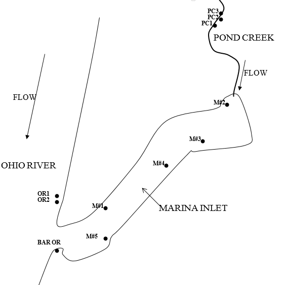
Figure 1: Schematic of sample locations.
In this report, a sediment budget analysis is being performed for the Louisville Yacht Club Marina in Louisville, Kentucky. Using a number of tracers contained within sediment at the Yacht Club location, we will be preforming an analysis to determine from which sources sediment is being eroded and ultimately deposited at the location of interest. We have identified the Ohio River and Pond Creek as sources in this analysis. Using samples form the Yacht Club and these two sources, we aim to determine through statistical means (t-testing) which tracers we can best help us identify the proportions of sediment from each source that are contributing to the total. Iron, Potassium, Nickle, and Zinc were identified as tracers that could be used in a simple unmixing model to ultimately identify the proportions of sediment being contributed to the deposition at the Yacht Club. This process concluded that roughly 30% of that sediment was contributed from the Ohio River, and roughly 70% was being contributed by Pond Creek. Leading to the conclusion of Pond Creek being the dominant source of sediment load production, using that we calculate the sediment yield for the marina.
Introduction
Increased sedimentation in small reservoirs can be detrimental to the local environment and benthic habitat for many organisms. Deposition of fine sediments can have severe ramifications on an ecosystem’s trophic level by blocking the accessibility of oxygen for macrophytes. Fine sediments within a water column can also reduce the amount of light penetration, inhibiting photosynthetic processes. An increase in sediment delivery to a local accommodation space may eventually increase flood potential due to the raised stream bed while reducing the water capacity.
The Louisville Yacht Club and Marina is impacted by sedimentation processes originating from the transport and deposition of fine sediments from the Ohio River and the conjoined Pond Creek tributary, a source of sediment originating from nearby construction sites (Figure 1). The Marina is located on the southern bank of river mile marker 593 of the Ohio River. It has been observed that during storm events, sediment is deposited within the marina, often requiring dredging remediation to maintain the function of the marina. The immediate stakeholders of high sedimentation impacting the Marina include the boat owners and the associated consultants who prescribe the dredging and remediation maintenance measures. By calculating the sediment budget for the marina and determining the sediment yield ratio for the sources, we can devise a plan of operation to control erosional processes provided by the dominant source.
Argument
Identifying sediment sources and the extent erosional processes can transport sediments in fluvial settings is essential for watershed management. Construction sites are notorious for being the source of large volumes of sediment that ultimately get deposited in local watersheds. Due to the surficial and invasive nature of construction processes, construction sites characteristically involve exposed soil due to the removal of topsoil and vegetative layer, loose soil from excavation operations, and possess no trees to provide this soil with canopy cover. The culmination of these factors lead to a severely elevated susceptibility to erosion by rainfall impact. According to Zech et al. (2009), more than 80 million tons of sediment are washed from construction sites in the U.S. each year. This process can bring on a number of issues such as reducing reservoir capacities downstream or negatively impacting the habitat and environment of organisms within the stream. Challenges posed by erosion from construction sites are approached by applying best management practices to the impacted sites (Zech et al, 2009).
Beighley et al. (2010) investigated the application of erosion control blankets which typically formed with compost. Overlying the exposed soil with compost blankets is a suggested approach to provide resistance against the erosive forces of runoff on the site. This study concluded that the blankets were effective in reducing erosion from runoff by increasing flow resistance and providing more time for the runoff to infiltrate the soil.

Figure 2: Scatterplots for elemental data relative to mixed Marina sediment compositions.
The Universal Soil Loss Equation, as discussed in Clark et al. (2009), is used as a predictive tool to be applied to construction sites. The variable outlined with the most value was Rainfall Erosivity (R) due to the relationship that it is independent of land use practices for these sites. The paper considers a study performed in Pennsylvania where researchers collected R values at various locations and compared their values with the ones provided by the USDA isoerodent maps. Their results revealed that the USLE underestimates the impact of rainfall for erosion estimates. Constructing sediment ponds and utilizing erosion control blankets were suggested to be the best methods for reducing the impacts of eroded sediments.
Adverse effects on aquatic biota, reduction of freshwater habitats, and decreasing microbial population are consequences of increased sedimentation (Zhang et al., 2012). Endemic to the Ohio River is the orange-footed pearly mussel, an organism that utilizes filter feeding at the sediment-water interface of the streambed. The mussel population is now endangered due to upstream construction activities and transport of fine sediments. Non-point source sediment delivery to sensitive aquatic ecosystems for grains less than 62 μm in diameter is considered to be the most prevalent pollutant in the U.S. (Davis et al., 2009).
Zinger and et al. (2011) studied extreme sediment pulses in the Wabash River in the Midwest. They discovered that each major stream discharge event triggered a rapid delivery of sediment from one to five orders of magnitude greater than those produced by lateral migration of individual bends. Much of the material produced by these events was deposited at the confluence of the Wabash and Ohio River. This study of meander cutoffs can be related to our study in the Ohio River where ultimately the sedimentation of the marina is caused by high discharge events that result in backflow as the raised Ohio River feeds back into the marina with slower flow velocity.
The impact of erosion processes that occur from upstream construction site operations increase with greater surface area of bare soil on these sites. Various design elements and BMP’s can be applied to properly planned areas from our sediment source project to significantly reduce the amount of sediment being transported to streams including silt fences, sediment ponds, and erosion control blankets.
Methods & Results

Table 1: Client provided data.
Sediment data was collected including inorganic elements and sediment bed deposition measurements. Inorganic elemental tracer data was collected at the source locations and mixture locations. In addition, depth of deposited sediment was collected at the mixture locations. The depth of deposition occurred over a 30 month period. Using the elemental data provided (Table 1) by the client, we were able to deduce the appropriate sediment tracers that differentiate the two sources of sediment impacting the Marina. The 12 tracers included Al, Ba, Ca, Co, Cr, Cu, Fe, K, Mn, Ni, Sr, and Zn. By creating scatterplots of the elemental data we can visually limit which tracers may be suited. From this selection, we performed T-tests to verify the tracers are statistically different.

Table 2: T-test.
From the scatterplots, we were able to surmise that Ni, K, Fe, and Zn are viable tracers to differentiate the sediment sources (Figure 2). To verify this interpretation, we performed T-tests. All 4 tracers proved viable because the T-values were more than the 2.5 value presented in the t-table (Table 2).
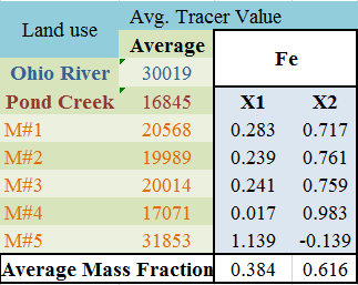
A simple un-mixing model was used to determine the relative sediment source contributions. With each tracer for the two sources, 5 mixing locations were considered to apply the model (Equation 1, Equation 2). The procedure was repeated several times and the average mass fraction was calculated.
T(mix) = X1T1 + X2T2 Equation (1)
X1 + X2 =1 Equation (2)
The following tables represent all results for the 4 tracers: Fe, K, Ni, Zn.
Tracer: Fe
As shown in Figure 3, X1 and X2 are equal to 0.384 and 0.616, respectively. Pond Creek contributes 61.1% and Ohio River provides 38.4 % for the iron content.
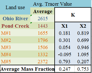
Tracer: K
As shown in Figure 4, X1 and X2 are equal to 0.247 and 0.753, respectively. Pond Creek provides 75.3 % and Ohio River contributes 24.7% load of the total potassium content for the sediments.
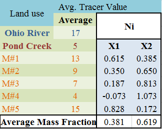
Tracer: Ni
As shown in Figure 5, X1 and X2 are equal to 0.381 and 0.619, respectively. Pond Creek supplies 61.9 % and Ohio River adds 38.1% load of the total nickel content for the sediments.
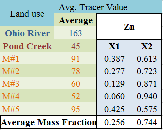
Tracer: Zn
As shown in Figure 6, X1 and X2 are equal to 0.256 and 0.744, respectively. Pond Creek provides 74.4 % and Ohio River supplies 25.6% load of the total zinc content for the sediments.
The next step would include a sediment yield calculation. To estimate our sediment budget, we implemented the Reservoir Method for calculating sediment yield for the 30 month duration of deposition. In order to perform a sediment budget for a watershed, we must estimate the mean total streambed storage by considering the approximate surface area, depth of sediment sampling, and fine sediment bulk density.
The area of the Marina’s water surface was calculated by creating a polygon using ArcGIS software. We found 31844.54181 m^2 to be the approximate area. According to the client. the time interval for deposition was 30 months. The mass of sediment in and out of the system will be derived from using the range of bulk density for sediment and an average volume given by measurements of sediment bed deposits. Bulk density of the sediment is assumed to be between 1.1 and 1.4.

The mass of sediment stored in the bed, mB, is estimated using the following equation: Equation (4).
Where VB is the volume of sediment in the bed equal to the surface area of the deposition zone (31844.54181 m^2) times its average depth and pB is the sediment bulk density in the streambed. The average depth of sediment deposition was found to be 64.4 cm.
Using these equations we found that between approximately 751.95578 meters^3 and 957.0346 meters^3 are being transported and deposited to the system on average per month.
Discussion
Assumptions considered in our analysis include assuming large scale variability was adequately accounted for in sampling of sediments at different locations within the watershed. The depth of stored sediment in the Marina deposits varies, indicating the dependence of sediment storage zones on the small-scale variation and control of geomorphologic features in the corridor. We assumed the control of these features were uniform throughout the basin. For our sediment yield equation, we are assuming conservation of mass applies within our reservoir and that there is no reworking of sediment out of the reservoir after it has first been delivered during this one month time interval.
The results reflected the literature well. Our dominant source contributing the most sediment was consistently the Pond Creek tributary due to its proximity to the construction site upstream and its episodic, flushing nature represented by the local hydrograph. The Ohio River contribution of sediment had a steadier, tidal effect on the marina. Most of the sediment entering the marina from the Ohio River most likely occurred when the Ohio River was at or near bankfull level.
This study could be very useful for other consultants that frequently must carry out dredging remediation operations in small watersheds. The best use for a client’s budget could go towards constructing sediment ponds and implementing silt fences and erosion blankets upstream near the construction site to dramatically reduce the sediment delivered to a storage area.
References
1. Zech W.C, McDonald J.S., Clement T.P. (2009)” Field Evaluation of silt fence tieback systems at a highway construction site”. Practice periodical on structural design and construction, ASCE. 14(3): 105-112.
2. Beighley R.E, Sholl B., Facette L.B, and Governo J. (2010).” Runoff characteristics for construction site erosion control practices”. J. Irrigation and drainage engineering, ASCE. June 2010: 405-413.
3. Clark S.E, Allison A.A, Stiler R.A. (2009).” Geographic variability of rainfall erosivity estimation and impact on construction site erosion control design”. J. Irrigation and drainage engineering, ASCE. July/Augest 2009:474-479.
4. Zhang Y. S, Collins A.L, Horowitz A.J. (2012). “A preliminary assessment of the spatial sources of contemporary suspended sediment in the Ohio River basin”. J.Hydrological processes, 26, pp: 326-334.
5. USGS Report “Results of a Two-Dimensional Hydrodynamic and Sediment-Transport Model to Predict the Effects of the Phased Construction and Operation of the Olmsted Locks and Dam on the Ohio River near Olmsted, Illinois”. Water- resources investigation report 03-4336, Department of the Interior, Geological Survey.
6. Davis C. M, M.ASCE, Fox J. F and M.ASCE. (2009). “Sediment fingerprinting: Review of the method and future improvement for allocation nonpoint source pollution”.135, pp: 490-504.
7. Belmont P, Gran K, Schottler S.P, Wilcock P, Day S. D, Jennings C, Lauer J. W, Viparelli E, Willenbring J. K, Engstrom D. R, Parker G. 2011. “Large Shift in Source of Fine Sediment in the Upper Mississippi River”. J. Environ. Sci. Technol. (45), pp: 8804-8810.
8. Collins, A. L., & Walling, D. E. (2002). Selecting fingerprint properties for discriminating potential suspended sediment sources in river basins. Journal of hydrology, 261(1), pp: 218-244.
9. Horowitz, A. J., Elrick, K. A., & Smith, J. J. (2001). Estimating suspended sediment and trace element fluxes in large river basins: methodological considerations as applied to the NASQAN programme. Hydrological Processes, 15(7), pp: 1107-1132.
10. Zinger, J. A., Rhoads, B. L., & Best, J. L. (2011). Extreme sediment pulses generated by bend cutoffs along a large meandering river. Nature Geoscience, 4(10), 675-678.
Spring 2016
Pioneer Paleolimnology Lab
A Holocene Paleoenvironmental Reconstruction of a Unique Amazonian Landscape using Lake and Ria Sediments
Motivation
The operation of the 5km-wide Belo Monte Dam in Altamira (Brazil) could flood up to 6000 km2 and force the relocation of 20,000 people from 18 ethnic groups and indigenous communities. In addition to the social injustice, the Belo Monte project is expected to result in a tremendous loss of biodiversity downstream in the Volta Grande do Xingu, including many endemic fish and reptiles. This study was performed to examine the environmental sensitivity of the region using lake sediment cores. We can use insights from the Quaternary to better understand how the Volta Grande riverine landscape has responded to changes in climate and hydrology. These results may help us predict potential aquatic ecological changes associated with dam emplacement and altered tropical river dynamics in the future.
Background

This study is centered on a 122 cm sediment core that was extracted from a floodplain lake within the Volta Grande, a large bend in the Xingu River upstream of the vast Xingu ria. The core represents a depositional record of the mid-Holocene to present (~7000 yrs). The Xingu River is a bedrock-dominated anastomosing river in the Altamira region, draining a watershed of ~510,000 km2. Controlled by tectonics, the river flows over Archean gneisses, Devonian shales, siltstones, and sandstones, and Triassic-Jurassic diabase before entering the Amazon sedimentary basin. At this transition, the river forms a sharp bend and generates steep rapids which harbor substantial endemic species, including catfish and stingrays. Stable sandbars, large rapids, and a series of anastomosing channels together generate the hydrological conditions that gives the Xingu River its rich biodiversity.
Methods
All samples were analyzed in 2 cm intervals and routinely quality checked with standards. Geochronological and magnetic susceptibility values were provided by University of São Paulo.
ED-XRF
Bruker Tracer IV-SD
Carbonate Coulometry
LECO
Magnetic Susceptibility
Geochronology
Radiocarbon (AMS)
Quartz OSL
Biodiversity
The Xingu River hosts a great variety of tropical freshwater fish; dam emplacement is predicted to set a record for biodiversity loss in this region. The Belo Monte Dam will impact the aquatic environment by blocking passages for migratory species, reducing flow velocity, and delaying seasonal flood pulses. Several endemic species of reophilic and armoured catfishes, including the cherished Hypancistrus zebra will be endangered as a result of the dam.
Results


The lake sediment core is interpreted to reflect three phases of depositional environment evolution in this upstream region of the Volta Grande do Xingu system. An integrated assessment of sedimentology, geochemistry, physical properties, and geochronological data indicates that topographic closure and lake formation began ~3900 yrs BP. Intriguingly, the inception of the lake phase immediately follows the famous 4.2 ka arid event that impacted much of tropical South America. Recovery of the monsoon in the late Holocene may have helped the basin maintain a positive water balance, as indicated by accumulation of organic matter-rich clays. Quartz OSL dating produced ages of 3090 ± 30 y BP at 15cm and 6840 ± 513 y BP at 120 cm. AMS produced a 4188 ± 378 y BP date for 84cm. General sedimentation rates were able to be calculated using these ages.
The core from the Xingu ria is much shorter temporal record (~1000 yrs in length), suggesting high sediment accumulation rates. Multi-indicator analysis has revealed the presence of high frequency “event layers” that stand out in sediment chemistry and magnetic properties. Our preliminary interpretation is that ria sedimentation is sensitive to large storms, and that the core may be one of the few records of late Holocene paleotempest activity in the lower Amazon. Future work on the age model will help clarify potential climatic forcings for these storms (e.g., solar activity, ENSO, etc).
Paleogeographical illustration of the Volta Grande near Altamira from ~7000 y BP - present. River appears blue, and the landscape appears green-brown (lighter, brown hues signify relative degree of aridity).


Conclusions
Lithofacies and chemostratigraphic data indicate a three phase evolution (fluvial → transitional→lacustrine) of depositional environments at the island lake site. The lake phase is marked by clay and organic matter rich sediments, whereas the fluvial environment (channel center bar and/or unvegetated island) are sandy and organic lean.
The inception of the floodplain lake occurs after the 4.2 ka arid interval in South America, suggesting that resumption of the summer monsoon may have been important for the evolution of this lentic ecosystem.
Farther downstream, the Xingu ria enters the Amazon sedimentary basin forming a single wide slackwater channel. Preliminary analysis of the ria core suggests high sedimentation rates and the potential for a late Holocene paleotempest record that will be explored in the future.
Natural factors influencing flow in the river clearly affect the surrounding environment, and changing the flow dynamics could alter ecological processes in severe ways.
References
Bertani, T. C., et al., (2015). Understanding Amazonian fluvial rias based on a Late Pleistocene–Holocene analog. Earth Surface Processes and Landforms, 40(3), 285-292.
McGlue, M. M., et al., (2012). Lacustrine records of Holocene flood pulse dynamics in the Upper Paraguay River watershed (Pantanal wetlands, Brazil). Quaternary Research, 78(2), 285-294.
Pérez, M. S. (2015). Where the Xingu Bends and Will Soon Break. American Scientist, 103(6), 395.
Sawakuchi, A.O., et al., (2015). The Volta Grande do Xingu: reconstruction of past environments and forecasting of future scenarios of a unique Amazonian fluvial landscape, Sci. Dril., 20,21-32, doi:10.5194/sd-20-21-2015, 2015.
Spring 2018
Exploring Channel and Topographic Characteristics Related to Tectonic Deformation in the Ruhuhu River Watershed, Tanzania
Introduction

Lake Malawi exhibited an open hydrologic system that was present even during dry, shallow periods prior to 800ka. Following the lake level transition around 700ka, the lake deepened and became more hydrologically closed with the exception of a single outlet, via the Shire River in the southernmost region. The most feasible candidate for an earlier outlet is the current influent and rift-antecedent Ruhuhu River (Ivory et al., 2016). It was hypothesized (Ivory et al., 2016) that an uplift occurred 700-800ka and altered the direction of flow in the river. For a given tectonic uplift, when one side of the tectonic divide rises, the other side is lowered which reduces the relative base level. After the uplift surfaced, the lake deepened until it reached the modern outlet in the Shire River, where it presently drains through the Zambezi River to the Indian Ocean.
Demonstrated by evidence found in the aquatic evolution of Lake Malawi, the present day Ruhuhu River inlet once served as the outlet and connected the rift lake to the Indian ocean (Ivory et al., 2016). By performing analyses on the Ruhuhu River watershed, we can determine if there are tectonic controls impacting the river’s flow behavior. Digital elevation models (DEM) provided by satellite imagery data will be utilized to assess the fluvial patterns and landform characteristics for evidence of tectonic deformation to test the hypothesis that a structural uplift in the Ruhuhu watershed was responsible for the change in Lake Malawi’s hydrology and biodiversity.
Methods

DEM map illustrating the northeast area of Lake Malawi overlain by the primary Ruhuhu River drainage network of HSO 5-8. Red-shaded areas represent low elevation and green-shaded areas represent higher relative elevation.
Digital elevation data studied in this project was obtained from the NASA Shuttle Radar Topographic Mission (SRTM) database that is distributed by USGS. The highest resolution data for eastern Africa has a 3 arc-second resolution (approx. 90m) and is formatted in 5 deg x 5 deg tiles. The files are georeferenced to the WGS84 datum.
All the data that was gathered for this project was processed and extracted using the terrain analysis and hydrologic modeling capabilities provided by the RiverTools software (version 4.0.2) by Rivix, LLC.
To test the hypothesis that the direction of flow in the Ruhuhu River reversed in response to a tectonic uplift, this study investigates several morphometric parameters to describe the watershed. The morphometric parameters utilized in this study include Asymmetry Factor, Elongation Ratio, Drainage Density, Hypsometric Integral, Shape Factor, Sinuosity, and Stream-Length Gradient Index. These calculations were made for 9 other subbasins identified in 4 zones of high drainage density on the north and eastern margins of Lake Malawi and also for the Ruhuhu drainage network and its 5 independent subwatersheds.
Morphometric parameters


Data

DEM map showing the location of zones and large basins evaluated for the Lake Malawi watershed.
Zones surrounding Lake Malawi were defined to split the large DEM file into smaller, more manageable sizes. For each of the 8 zones defined, the largest HSO streams that had outlets at the lake margin were designated as a basin. Channel profiles were extracted for the largest order reach of the stream. Relief along this profile, profile length, slope, and sinuosity were all measured for these main drainage lines. Additionally, if the stream had one or two large tributaries of one HS order less than the main channel, the criterion was also evaluated for them. When evaluating the drainage network that supplies Lake Malawi, there were no significant basins contributing to the lake on the eastern perimeter except LMZ8, the Ruhuhu River watershed. That is why there are no watershed characteristics described for zones LMZ5-7. LMZ4 basin characteristics are listed as CP12 because there are two large order streams that make up a single basin in LMZ4. The Ruhuhu Watershed, LMZ8, is the only basin that is further divided into subbasins. Watershed analyses was performed on the entire basin (LMZ8Ruhuhu) draining to the main HSO 8 - Ruhuhu R. drainage line and for the 5 tributaries of HSO 6 or 7, LMZ8_CP1-5.
Results
The area was calculated south of the east-west trending channels of the main Ruhuhu River and its tributary referenced as LMZ8_CP3 to determine the asymmetry factor. The area of the Ruhuhu watershed south of this line was approximately 6064 sq. km. Ruhuhu River drainage was shifted towards the downstream southern side of the main drainage line.

Asymmetry Factor (Af). Given by area south of main drainage line in relation to the total basin area. Black arrows point in the direction of basin tilt.
In the basin relief vs. CDF HI plot, Z8CP1 and Z8CP2 basins have high relief values and high CDF HI values. This relationship is characteristic of less mature networks. Z8CP3 and Z8CP4 basins have low relief and CDF HI, indicating these basins are more mature and stabilized. Z8_CP5 and the whole Ruhuhu R. watershed have high basin reliefs and low CDF HI values. The graph illustrating Basin Relief against the elevation-relief ratio method for HIS has a more obvious trend line for the two basin zone categories compared to the basin relief vs. CDF approach to HI.
The slope vs. sinuosity plot reveals that the Ruhuhu subbasins and other basin zones have opposite relationships. As slope increases in the main channels of their respective Ruhuhu subbasins (Z8CP1-5), sinuosity decreases. However, for the HSO 8 Ruhuhu River, there is a very low gradient accompanied by a very high sinuosity. Basin relief plotted against sinuosity demonstrated that the subbasins of the LMZ8_Ruhuhu basin categorically have higher sinuosity compared to the LMZ1-4 basins despite having large basin relief.
Any SL index computed for an entire channel length will simply be equal to the channel’s change in elevation. SL was only computed for 4 segments within the Z8_Ruhuhu basin. Each of the 4 segments proved to have significantly high SL values, emphasizing how sensitive drainage networks and channel profiles are to knick points.
Demonstrated by the elongation vs. drainage density plot, the Z8Ruhuhu subbasins skew slightly more elongated than the other zones. Z8CP1 and Z8CP3 are significantly more elongate than the rest. The Ruhuhu R. watershed has lower values of drainage density compared to other basins, illustrated in the shape factor and drainage density plot.


Discussion
The values reported for the basin relief vs. CDF HI plot suggests the uplift event most likely occurred on the north/northwest area of the Ruhuhu watershed and tilted the basin south of the main channel (Ruhuhu: HSO 8). The highest values for SL index of the four channel reaches tested occurred in the main channels of the Z8CP1 and Z8CP2 basins, 797 and 880 respectively. The latter is especially important because it occurs just upstream of the CP2 and Ruhuhu R. confluence, which is also immediately downstream of the Ruhuhu’s second water gap. Because Z8CP1 exhibits high basin relief, high sinuosity, high CDF HI, a high elongation ration, and low shape factor, the uplift event most likely originated within close range of this basin.
A river will try to maintain its channel slope so when there is an uplift, the downstream side of the uplift will have been raised and have a steeper valley slope. In response, the river channel increases sinuosity to preserve its original channel slope. The area upstream of the uplift will straighten and decrease sinuosity since the overall stream valley slope has decreased. If the valley slope increases in the opposite direction, a normal fault has downthrown the upstream side resulting in downstream straightening and incision (Zamolyi et al., 2010).


Conclusion
Ruhuhu River Watershed.
Various geomorphic parameters describing watershed responses to tectonic uplift were quantitatively measured and spatially evaluated to determine if a tectonic origin is responsible for the topographic and drainage network expression within the Ruhuhu watershed. The data collectively demonstrates that the westward flow of the Ruhuhu River is a fluvial response to a tectonic uplift that constrained the basin perimeter to its present day location. Watershed characteristics for the Ruhuhu basin and its subbasins revealed relationships associated with structural influence. Nine other inlet basins of Lake Malawi were evaluated similarly and plotted with the Ruhuhu watershed values. This allowed me to distinguish how much the Ruhuhu is influenced by certain attributes in comparison to other similar, more stable bedrock rivers in the same geographic setting. Apart from the numerical assessment, the delineated Ruhuhu watershed exhibits some eastward directed tributaries and also heavily incised meanders, observed through Google Earth. The exact location of where the uplift occurred is unknown. However, given the presence of two large water gaps along the main channel of Ruhuhu R., the rate of incision outpaced the local rate of uplift.
References
Cohen, A. (1990). Lacustrine Basin exploration-case studies and modern analogs. In AAPG Memoir 50.
Doranti-Tiritan, C., Hackspacker, P. C., de Souza, D. H., & Siqueira-Ribeiro, M. C. (2014). The Use of the Stream Length-Gradient Index in Morphotectonic Analysis of Drainage Basins in Pocos de Caldas Plateau, SE Brazil. International Journal of Geosciences, 5(11), 1383.
Eccles, D. H. (1974). An outline of the physical limnology of Lake Malawi. Limnology and Oceanography, 19(5), 730-42.
Gaidzik, K., & Ramirez-Herrera, M. T. (2017). Geomorphic indices and relative tectonic uplift in the Guerrero sector of the Mexican forearc. Geoscience Frontiers, 8(4), 885-902.
Ivory, S. J., et al. (2016). Environmental change explains cichlid adaptive radiation at Lake Malawi over the past 1.2 million years. Proceedings of the National Academy of Sciences, 113(42), 11895-11900.
Ket-ord, R., Tangtham, N., & Udomchoke, V. (2012). Synthesizing drainage morphology of tectonic watershed in upper ing watershed (Kwan Phayao Wetland Watershed). Modern Applied Science, 7(1), 13.
Mahmood, S. A., & Gloaguen, R. (2012). Appraisal of active tectonics in Hindu Kush: Insights from DEM derived geomorphic indices and drainage analysis. Geoscience Frontiers, 3(4), 407-428.
McCullough, G. K., Barber, D., & Cooley, P. M. (2007). The vertical distribution of runoff and its suspended load in Lake Malawi. Journal of Great Lakes Research, 33(2), 449-465.
Molin, P., Pazzaglia, F. J., & Dramis, F. (2004). Geomorphic expression of active tectonics in a rapidly-deforming forearc, Sila massif, Calabria, southern Italy. American journal of science, 304(7), 559-589.
Pike, J. G. (1968). The hydrology of Lake Malawi. The Society of Malawi Journal, 20-47.
Rebai, N., Achour, H., Chaabouni, R., Kheir, R. B., & Bouaziz, S. (2013). DEM and GIS analysis of sub-watersheds to evaluate relative tectonic activity. A case study of the North-south axis (Central Tunisia). Earth Science Informatics, 6(4), 187-198.
Singh, T. (2008). Tectonic implications of geomorphometric characterization of watersheds using spatial correlation: Mohand Ridge, NW Himalaya, India. Zeitschrift fur Geomorphologie, 52(4), 489-501.
Spring 2017
Mentor: Dr. Jonathan Phillips
Stream Channel Responses to Increased Nonpoint Source Pollution: A Spatial Analysis of Red River Gorge Watershed
Introduction
Throughout the state, the Kentucky Division of Water has recognized several watersheds in need of urgent restoration (Figure 1). This status is a result of at least one nonpoint source pollution such as urban runoff, failed septic systems, agriculture, and surface mining. Among this list is the Red River Gorge Watershed, covering ~148 mi^2. Within the drainage area, pathogens introduced by illegal dumping, loss of streamside vegetation, erosion, and runoff from towns, fields, surface mines, and mills threaten public health. KDOW has attributed the poor water quality to sources of increased sedimentation, impairing the aquatic habitat of local headwater tributaries. This project aims to define probable cause of increased sedimentation to unregulated outdoor regulation and other regional land uses as a function of the regional geology. Evident in Figure 2 and Figure 3, most portions of USFS designated trails lie on the more resistant upper Mississippian and Pennsylvanian formations. In Figure 4, however, the trails lying among seemingly resistant strata are actually lying amid a very expansive region characterized by risk of landslides and slope instability. Figure 5 illustrates the regional surface gradient, supporting the risk of slope failures as well as showing the range of elevation the trails actually occupy. In Figure 2, concentrations of barren land and forested regions provide evidence for trail popularity, land use, and stream channel responses to increased sedimentation sources. Where the park is largely accessible, there will be increased impacts of downstream aquatic habitat impairment, sediment production, runoff, and bank destabilization.


Methods
Assembling data of varying file types, sizes, and projections required performing different functions available in ArcGIS 10.1 including georeferencing, selecting by attribute, projection transformations, spatial joins, and extracting by mask. Using the slope function under spatial analyst tools was required to derive slope values for the DEM raster dataset. The statistics function was utilized to obtain stream and trail mileages within each sub-watershed.
Struggles to adequately represent the necessary data originated in the difficulties to locate applicable data online. Once the represented data was downloaded, problems georeferencing certain images and complications overlaying various files arose. Ultimately, it was determined that the desired overlays would only provide statistical data for different features present in their respective watersheds, information that is often considered inherently obtuse when investigating fragile ecological relationships. The affinity of one feature to another could be made with probable cause due to geographic distribution of spatial characteristics. Failure to georeference a pertinent Red River Gorge Forest Service Map prohibited the creation of a park boundary polygon, as well as a shapefile representing roads throughout the region. A Red River Gorge Geological Area map boundary would have added an appreciable reference to the region and spatial relationships in question; however, references to the land cover, geology, and USFS designated trails provides us with the opportunity to draw the same conclusions.
Data for the various representations of hydrology originated from sources including the Kentucky Geological Survey’s Geospatial Data Library, Kentucky Division of Geographic Information (KDOGI), Kentucky Division of Water, Kentucky Energy and Environment Cabinet, and the National Hydrologic Dataset provided by the USGS. These provided figures for the illustration of Kentucky River Basins, Major Rivers of Kentucky, Priority Watersheds, Stream Hydrology by County, and Hydrologic Units for Sub-Watersheds. Pertaining to the geographic units, the Kentucky state polygon was sourced from KDOGI and the Menifee-Powell-Wolfe County boundaries were collected from the KGS. The surface data by which many of the relationships have been based on originate from a host of sources involving a Simplified Geology of Kentucky file by KGS, 10 Meter DEM Elevation Service of Kentucky by USGS, Land Cover by the USGS and MRLC consortium, and designated trails provided by a USFS forest service map.
Discussion
Concentration of barren land are in proximity to Tunnel Ridge Road along popular and accessible trails, specifically the initial stretch of the Gray’s Arch Trail, around the junction of Auxier Ridge and Courthouse Rock Trails as well as ~200 ft. below this ridge-top section accompanying an upstream portion of a Red River headwater branch (Fish Trap Branch). Portions of barren land are also exposed on the gentle low gradient hillside immediately north of Nada Tunnel, a particularly sinuous part of the Ky 77 Scenic Byway [roads not illustrated]. A patch of barren land is also recognizable along the Rush Ridge Trail, specifically at a scenic viewpoint [trail names not illustrated]. Excessive foot traffic and visitor occupancy at these sites merely erodes the top surface of the ridge-line trails of resistant sandstone by disengaging ridge-top vegetation, allowing for any barren landscape exposure to be limited to the confined spatial extents of increased activity. High levels of recreational tourists in the region begin to increase sedimentation processes when the trails come in direct contact or close proximity to streams and regions of high grade topography. Though not as common within park boundaries [park boundary not illustrated], appearances of the pasture/hay land classification described by grass dominated vegetation, tends to lie adjacent to roads and alongside streams. Proximity and clustering of vegetation along streams could simply represent floodplain extent; however, it’s worth noting that just as the Red River leaves Menifee County and flows west into Powell County, the sinuosity of the channel increases abruptly along with the grassy vegetation occurrences. This is most likely occurring in response to a simultaneous drop in elevation, forest type, and geological unit transgression. Higher degrees of sinuosity are a function of greater volumes of sediment storage. Major accumulation of the grass-vegetated land increases with distance radiating from Red River Gorge boundary [boundary inferred in difference in Land Cover and is even more concentrated in regions that are more densely populated. This could be explained by an increase in neighborhoods, or similarly an increase in residential lawns.
Given by the land cover map, evergreen forest occupancy is constricted to the Clifty Wilderness region of the Red River Gorge Geological Area among the Clifty Creek and Swift Camp Creek Sub-watersheds. While it is safe to assume that increased human disturbance within a forested region would account for more degraded water qualities, the swift camp creek region of the gorge is least accessible and least popular. This is probably why the evergreens have remained populated there. However, the swift camp creek watershed also has the highest levels of pollutants. This can be attributed to city of Campton [not represented] that lies just southeast of the watershed. There, increased runoff and failed sewage systems have been identified as the prime contributors to the impaired water quality.
Fall 2015
Mentor: Dr. Jonathan Phillips
Quantifying Sediment Storage in the Red River Gorge Geological Area, Ky using Field Methods
Introduction
Involvement in recreational activities is growing in popularity. In 1999, a national survey revealed that hiking was the most popular form of outdoor recreation engaged by 67% of Americans (Cordell, 1999). In 2012, the outdoor recreation economy grew 5% annually between 2005-2011, a time of economic recession when many industries contracted. The importance of understanding the connection of land use and presence in the environment is increasing as the efforts to preserve forested and wild lands are impacted by encroaching development and rising tourism. Characterized by its geology and sandstone arches, Red River Gorge Geological Area is internationally recognized for its rock climbing opportunities. Red River Gorge is a National Natural Landmark and Historic District of Daniel Boone National Forest, comprising several congressional designations including a National Wild and Scenic River, National Scenic Byway, and Wilderness. Described by the geographic distribution of geologic formations, the overall rugged terrain and erodible shale and siltstone units support high levels of natural erosion without human disturbance. The purpose of this project was to estimate the bed load sediment storage of point bars (Figure 4) along the most popular stretch of the river and be able to make interpretations on the intensity unregulated hiking and camping activities have on the river’s channel stability and erosion.
Methods
Figure 3. Example of recent slope failure due to channel widening and bank instability given by fallen tree.
The site for the study was located in the Gladie Creek sub-watershed, along a 3 kilometer stretch of the river in the most popular and visited part of the forest given the proximity to KY 77, Sheltowee Trace trail, Jump Rock swimming hole, and Gladie Visitor Center (Figure 7). The site was selected in an effort to portray large local sediment storages as being a function of visitor occupancy. Determining bed load sediment storage of the river was done by measuring the length, mean width, and approximate height above the channel bed on point bar exposures along the banks (Figure 1). In addition to these notes, the presence of a log jam was noted if it appeared support causation of the point bar formation (Figure 2). This data was later compared to the daily mean discharge values provided by the USGS Red River Gage Site, approximately 27 miles upstream (horizontal distance of 9 miles) to account for the extent flow related point bars are exposed. For both data collection periods, the stretch of river covered was approximately equal in upstream and downstream distance of the Sheltowee Trace suspension bridge.
Figure 4. Large point bar in proximity to two heavily visited trails and nearby swimming hole. Floodplain also exhibits slope failure along the boundary of the point bar.
Results
A range of grains sizes from silt to large gravels 4-6 inches in diameter are evident along all parts of the studied portion of river, representing a sediment transport capacity that frequently varies as a function of stream discharge. Numerous log jams are evident along the river, collecting other woody debris and diverting flow and providing an environment for sediment accumulation. Also along the river are several extensive displays of tree root exposure (Figure 5), soil creep, and recent slope failures (Figure 3). For both data collection periods, the stretch of river covered was approximately equal in upstream and downstream distance of the Sheltowee Trace suspension bridge. Surface area of point bars during the weekend of low discharge expressed a cumulative 31,983 sq. ft., while the higher discharge data collection period was displayed a meager 11,749 sq. ft. surface area. Upstream values characterized by the 41 cfs mean daily discharge represented 215,257 ft^3 of sediment storage, while downstream values characterized by 6.1 cfs of discharge represented 242,200 ft^3. Volume of sediment for the upstream segment does not include Site 13, as it was determined to be a low lying floodplain given the large amounts of shrubby vegetation.
Figure 5. Common elaborate and extensive root exposures indicate future slope failures and bank widening.
Discussion
The resulting data and the surrounding steep topography indicates a sensitive relationship between discharge and sediment storage exposure, a product of the wide channel planform. Further, rare intermittent periods of high or peak discharge that occupy greater portions of channel width erode the bank sides intensively promoting bank failures, transmitting large woody debris and accumulating large volumes of sediment settle in point bars and along the bed as the river returns to lower mean discharges. Bank slope instability is caused by soil compaction from heavy trail and campsite visitation. Soil compaction, especially along river banks, extremely degrades slope stability by damaging riparian vegetation that requires less compacted soils to support the root structure that ultimately preserves and stabilizes channel widening.
Figure 6. Small tributary (unrecognized by current NHD datasets) lies along a region that experiences little to no recreational use due to distance from trails. Deeply incised and meandered, the stream supports the conclusion that accessible and popular regions of the forest reduce slope stability and increase channel width, contrasted by this image.
Inaccuracy of the data presented can be attributed to difficulty in estimating river depth at each site and constrained data given by the short segment of river measured, both of which are due to lack of proper equipment for river navigation. The season during which field work occurred also limited amount of data by the duration of daylight. Discerning between river transported sediment and slope failure present at a site was difficult. While they are both representations of upslope sediment sources, the study emphasizes the importance of sediment transport capacity and sediment storage that has been suspended and deposited by the river. During the course of the study, the method for measuring storage height was questioned on the basis that sediment (belonging to a point bar) along the wall of the current flow, or beneath the water surface should serve as a feature belonging to the cross-sectional channel form instead of being included into the height measurement. This doubt of sediment function was abandoned once it was realized that sediment belonging to a storage body or channel bed are both river transported deposits and products of channel aggradation.
Conclusion
Intensity of erosion and sedimentation along the stream will decrease with increasing distance from hiking trails and the KY 77 scenic byway, as use and frequency of visitation are strongly correlated with accessibility (Figure 6). Given the observed topographic and geologic relationships of the region as well as measurements of bed load sediment storage and erosional features, the Red River evaluated in the study exhibits widening and aggradation, two stages of channel adjustment. And finally, despite the data being collected from a restricted 3 km stretch of the river, there are no major local variations in geology or land use giving rise to the generalizations made about erosional impacts of hiking trails are likely to be relevant to all portions of the river in proximity to recreational practice.
Fall 2017
Mentor: Dr. Frank Ettensohn
DESCRIBING THE HISTORY AND ORIGIN OF CARBONATE MUD MOUNDS IN SOUTHERN KY
The objective was to determine the history and origin of facies present in a specific carbonate mud mound outcrop in south-central Kentucky. By integrating our knowledge of the regional geological history of the Neoacadian Orogeny, concepts of basement uplift and sea level transgression, and sediment delivery mechanisms that might have existed in the channel at the time of deposition, we could incorporate field observations to determine the origin of the structure. Field observations involved characterizing representative sections of the outcrop, measuring, describing, and photographing the exposed area. Sedimentological, paleontological, and stratigraphic data including lithologies, biogenic structures, fossil fragments, and textures were carefully noted. The field notes were used to develop a representative stratigraphic column.
Study Site
Map of faults in eastern to south central Kentucky. Stops 9 and 10 mark approximate location of Burkesville outcrop. NW-SE trending faults are Precambrian in age and were reactivated by later orogenies. (Ettensohn et. al., 2012)
South-central Kentucky
~8.5 miles N of Burkesville, KY
Latitude: 36° 54′ 0.6″ N; Longitude: 85° 25′ 46.74″ W
Objective: Determine history and origin of facies present in the carbonate outcrop
Geologic Setting & Paleoclimate
Neoacadian Orogeny
Basement Uplift
Sea Level Transgression
Sediment Delivery via Borden Delta Channel Network
- Environment changed with adjusted sea level evident by multiple mud mounds “stacked” separated by glauconitic shales
- Mounds thicken on flanks due to storms wiping away tops of mounds and depositing crinoid debris in low stable areas
- Syntectonic deposition as noted by less displacement up-section and angular unconformity at bottom contact of larger mud mound
Thin Section Evidence
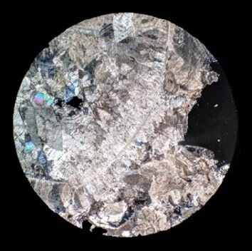
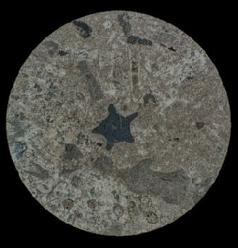


Conclusions
Regional effect of tectonics caused flexure and foreland basin development with associated foreland bulge due to subducting plates in the east
Rising of basement floor closer to photic zone allowed some sediment bafflers to establish in substrate at the inception of basin formation
The formation as a whole developed just before the delta complex completely was abandoned after a long phase of intermittent sea level regression
An alternate hypothesis could be that the mounds are deep water chemotrophs, but there is less evidence in this from the facies
A second alternative hypothesis is that these could be associated with turbidity currents that escape slope channels and got reworked by other currents into mounds
References
Ettensohn, F.R., Lierman, R.T., Udgata, D.B.P. and Mason, C.E., 2012, The Early-Middle Mississippian Borden-Grainger-Fort Payne delta/basin complex: Field evidence for delta sedimentation, basin starvation, mud-mound genesis, and tectonism during the Neoacadian Orogeny, The Geological Society of America Field Guide, v. 29, p. 345-395.
Greb, S.F., Potter, P.E., Meyer, D.L. and Ausich, W.I., 2008, Mud Mounds, Paleoslumps, Crinoids, and More: the Geology of the Fort Payne Formation at Lake Cumberland, south-central Kentucky, Kentucky Chapter of the American Institute of Professional Geologists Field Trip Guide, p. 1-45.
Paleogeographic map showing Borden Delta Complex and location of shoreline during Early and Middle Mississippian (Ettensohn et. al., 2012)
Stratigraphy of Fort Payne Formation and accompanying units (Greb et. al., 2008)
KY Highway 61 runs parallel to outcrop.
Field Evidence
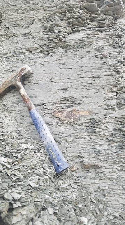


Credit: Clay Seckinger